
Cut your losses short, and let your profits run.
For centuries, that’s probably the number one trader’s adage. This is exactly what the trend following (TF) investment discipline does – using simple rules to be long markets in uptrends and short markets in downtrends. The mathematical rules used to identify uptrends and downtrends are predefined and mechanically implemented to eliminate human emotions in deciding when to be in or out of a market.
The most common way trend following is implemented is with managed futures funds, which are typically placed in the “alternatives bucket” of an investment portfolio, perhaps making up 5% of the total.  A good example of such a fund is the AQR Managed Futures Strategy Fund (Symbol: AQMIX). Managed futures funds apply the trend-following discipline to various equity and fixed income markets, along with currency pairs and commodity futures.
In this blog, I’ll examine the trend-following approach applied to asset classes that have a positive risk premium above inflation and T-bills, which are stocks and bonds. In addition, the focus will be to shift into cash when stock and bond trends are down, rather than more aggressively shorting downtrends. This is traditionally the realm of market timing, hence my distinction using the title “Trend-Following Market Timing”.
It’s an open question for me about whether managed futures funds add value over the long term, and this is worthy of a future blog piece. Generally, shorting stocks on a TF signal doesn’t work very well in the long term, but it does reduce managed futures fund correlation to stocks, and provides “bear market insurance” for a diversified portfolio of stocks and bonds. If you believe, as I do, that currency pairs and commodity futures do not deliver a long-term return above T-bills, then what kind of return can we expect from applying a trend-following overlay to these markets? I’m not sure what the answer is, so I won’t be addressing that question in this blog.
Everything I write beyond this point about trend following applies to the market-timing view of shifting between stocks and cash, and asking whether such an approach provides any sort of trading edge.
I love trend following. It fits my investment personality. When stocks are trending down, I can’t help but reduce my exposure to limit the downside. While reducing risk of loss, TF also reduces long-term returns, but that’s the investment discipline I’ve chosen for myself. Within the TF framework, I search for trading edges to enhance risk-adjusted returns, which is what this blog is all about.
While I’ve always been a trend follower for myself, I also see the logic of managing a portfolio in a buy and hold manner with an efficient markets view. As discussed in previous blogs, this approach to investing is hard to beat and is the most logical path to enhancing wealth over the long term. If I were leaving Earth for 10 years, with no access to my investment portfolio, I’d just hold stocks.
I was very fortunate to find Paul Merriman when I entered the investment management field. Trend following also fits his investment personality. In 1983, he founded the wealth management firm Merriman, where I’ve worked since 1999. At Merriman, our primary approach to managing client portfolios is to take an efficient markets long-term view using a diversified mix of low-cost stock and bond mutual funds.
But Merriman is unique in also offering trend-following programs because there’s a subset of clients where TF is a perfect fit psychologically. These investors know they can be highly susceptible to selling stocks emotionally during bear markets. Rather than shoehorning such a client into a buy and hold approach with a low equity exposure (such as a 30% stocks, 70% bonds), we can use a TF investment approach that ultimately delivers much higher equity exposure over a market cycle, thus providing higher investment returns. As is always the case, finding the investment discipline that best matches your psychological makeup is the first step in achieving investment success.
In this blog, we’ll test a few simple trend-following systems on the most liquid asset class with the longest low-transaction cost data history – the S&P 500. Next, with these results in mind, I’ll discuss what should be expected from trend following in the future. Lastly, I’ll discuss why the TF discipline can be attractive for investors and asset class traders.
Time Frame Selection
To examine the effectiveness of trend following, I backtested two TF systems on the S&P 500 over the time period of 1984 to 2014 (31 years). There are a few reasons I use the S&P 500. First, during this time frame, it was the most liquid and competitive market in the world, perhaps second only to U.S. treasury markets by these measures. S&P 500 futures were introduced in 1982, so the index was tradable at low cost over the entire time period. For this reason, we’ll neglect trading costs.
Secondly, we can expect that the S&P 500 was probably efficient to most, if not all, price-only trading systems during the entire period. Very low trading costs enabled the implementation of such trading systems. I’ve seen many studies using S&P 500 and Dow Jones Industrial Average daily data going back to the 1950s, the 1920s, and even back to the 1800s, using monthly data. While I understand the desire to go back as far as possible, backtesting TF systems on pre-1980s data has a number of subtle positive biases that artificially inflate risk-adjusted returns.
What’s wrong with the pre-1980s data? Before the 1980s, there was no trading vehicle to conveniently buy and sell the S&P 500. Yes, TF could have been implemented with individual stocks, or a basket of individual stocks, but this is not the data series used for backtesting. Any untradable index, including the S&P 500 Index or the Dow Jones Industrial Index has stale pricing and/or serial correlation in the data series. This effect enhances backtested trend-following performance. Once trading vehicles are introduced, these effects are immediately eliminated.
Commissions, spreads and taxes were also quite high in the old days. Pre-1980s traders were just as clever as traders are today. I’m sure many worked out the math and determined that TF returns after all costs were not that attractive at that time. Thus backtesting with this data has an additional implied assumption that we have a cost/trading vehicle advantage over other traders, which is absolutely not true going forward.
I’d rather use the shorter data series and logic to make a fair assessment of trend following than use the longer data series infected by positive biases. I expect the results shown next will be representative of what to expect from TF in the future, and what to expect trading ETFs and futures contracts associated with the myriad of asset classes currently available.
S&P 500 Trend Following Results
I use daily S&P 500 Index and yield data from 1983 to seed the TF systems, and as part of the study period from 1984 to early 1993. I’m relying on the futures-cash arbitrage mechanism to eliminate stale price effects and accurately reflect price behavior had an actively traded ETF existed during this time frame. From January 29, 1993, through 2014, I use daily data from an extremely liquid S&P 500 ETF (symbol: SPY). For a full description of the assumptions used in this study, see the disclosure below.
The TF models tested are the simple moving average (SMA) system and a channel breakout system. The SMA system is tested with five look back periods (LBP) of 100, 125, 150, 175 and 200 days. Trades are implemented at the close of the next day after a trading signal. When in cash, a three-month T-bill yield is used to simulate treasury money market returns. The channel breakout system buys when price breaks to a new x-day high, and sells when the price breaks a new x-day low; otherwise, the system makes no changes. I examined look back periods (x) of 40, 60, 80, 100 and 120 days.
These LBPs are chosen to exploit 6 to 12 month intermediate-term price movements to capture major up trends and side step major bear markets. Over this parameter space, the SMA system averaged 2.9 to 5.7 round-trip trades per year. The channel breakout system averaged 0.5 to 2.1 round-trip trades per year. Shorter LBPs have historically done poorly, so they’re not shown in this study.
I’ve tested many other trend-following models, including those with multiple and adaptable parameters. Their performance is very similar to the systems described above, plus there is no fundamental reason why these models should do any better than the two I tested.
Figure 1 shows the trend-following, risk-adjusted performance compared with a few benchmarks, and also mixes of stocks and bonds, and stocks and cash. Some TF return data points are above the stock-cash line (the red line), which indicates that if someone had used that system on the S&P 500, they would have added risk-adjusted value over the 31-year time period.
There are also parameters with results below the stock-cash line. How would you know ahead of time which LBP to use? Obviously, the answer is that you couldn’t have. Since all the LBP parameters appear reasonable, I tend to glaze my eyes and look for the centroid of all the data points. The result is not much different than a marker on the stock-cash line. Perhaps that’s what would be expected.
Figure 1: Simulated trend following returns on the S&P 500 Index from 1984 to 2014
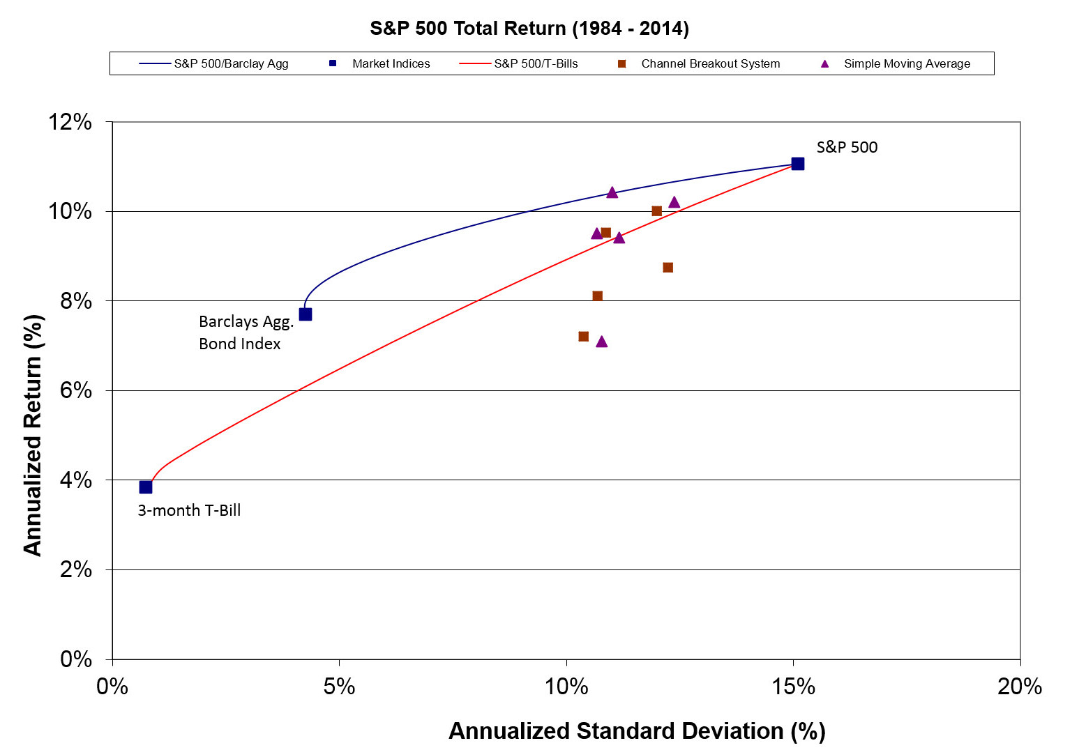
Comparing returns to a conventional stock-bond portfolio proves to be a higher hurdle because bonds beat cash over the long term. The last 31 years were particularly good for bonds, with interest rates falling over the entire period. We don’t expect the Barclays Aggregate Bond Index to outperform T-bills by almost 4% per year as was done during this time period. Looking forward, I’d expect the bond index to produce returns ~1-2% per year above cash.
Figure 2 shows the results with worst drawdown as a risk measure. At Merriman, we often use the rule of thumb that trend following cuts the standard deviation by a third, and cuts drawdowns in half. Using the glazed-over-eyes approach, it appears that the centroid of all the points appears to be above the stock-cash line. It seems reasonable to say that TF may add risk-adjusted value in the future when drawdown is the risk measure. This will be the case as long as standard deviation is the dominant risk measure used by investors and academics.
Figure 2: Simulated trend-following returns on the S&P 500 Index from 1984 to 2014, with worst drawdown as the risk measure
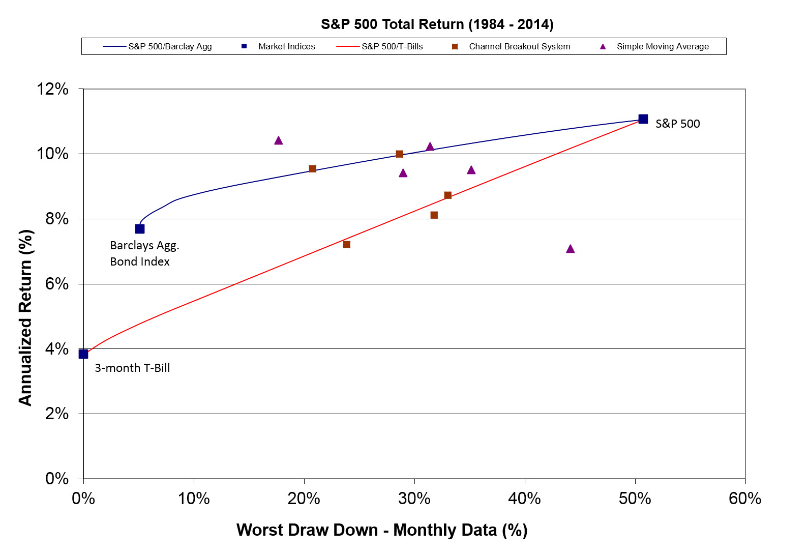
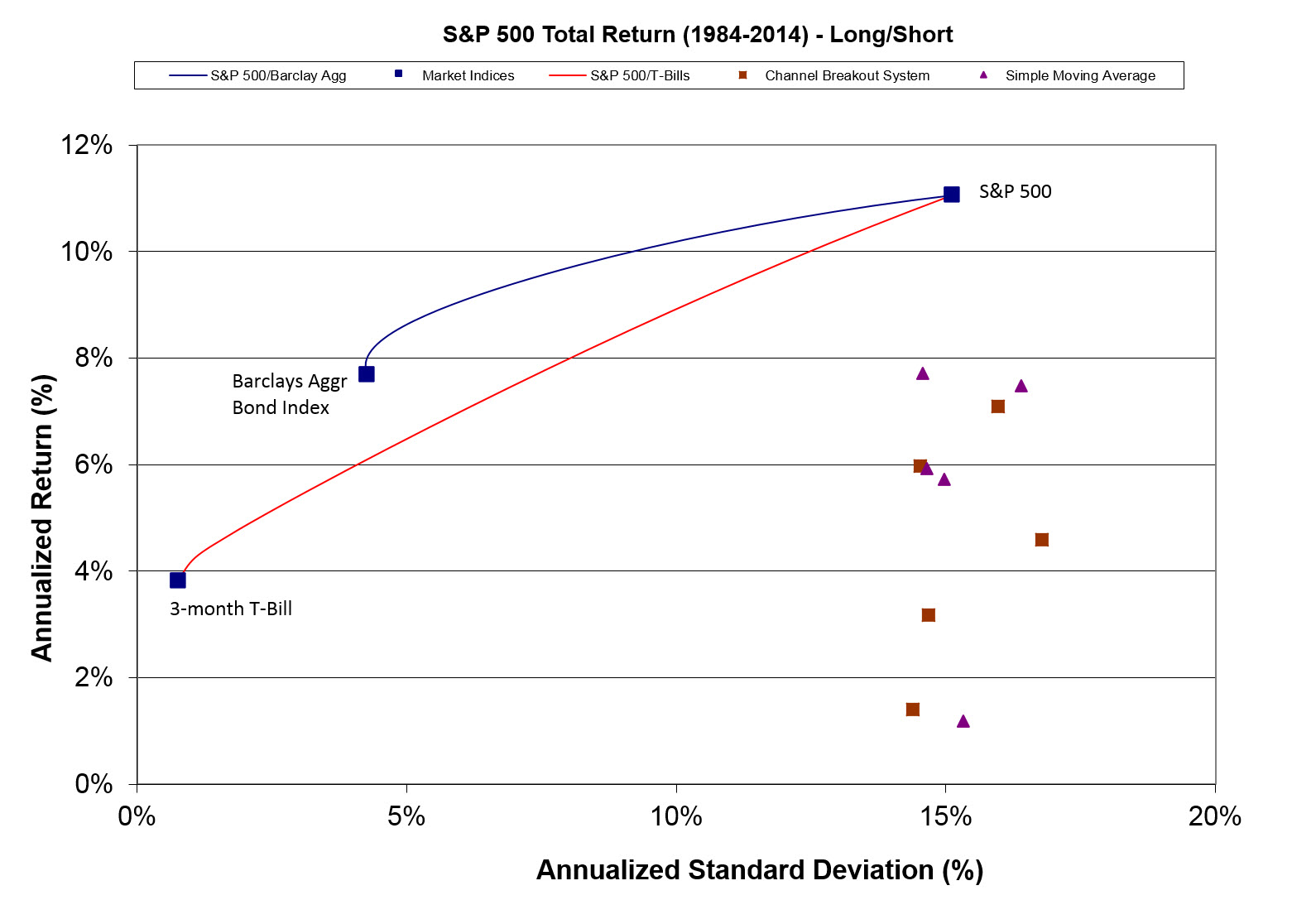
Figure 3 shows the TF returns when going long-short the S&P 500 rather than shifting to cash when a downtrend is signaled. The results are not very good, undoubtedly because the S&P 500 tends to rise in value when TF models signal downtrends.
The correlation of trend-following system returns to S&P 500 returns ranges between 0.7 and 0.75, rising as the LBP is raised. Using the long-short TF approach drops the correlation to between 0 and 0.25, again rising as the LBP is raised. Managed futures funds typically go long-short, and this helps reduce the correlation to the S&P 500, which is highly desired by institutional investors. Obviously mixing in TF applied to uncorrelated markets in fixed income space, currencies, and commodities will further reduce the correlation to 0, as is historically observed.
Figure 3: Simulated trend-following returns on the S&P 500 Index from 1984 to 2014 using a long-short approach
The bottom line from the backtested results is that there is no alpha derived by applying a TF system to the S&P 500 using standard deviation as the risk measure. So let’s talk about implications, nuances and generalizations for trading asset classes.
Future Expectations
What lessons can be learned from the above analysis?
Repeated studies like this, efficient markets logic, practical experience and low barriers to entry all suggest that trend following is not an alpha source, at least with respect to trading between the S&P 500 and cash. In the long term, I expect intermediate-term trend following to produce a risk-return profile that’s near the stock-cash line, which will be slightly inferior to holding a mixture of stocks and bonds. This view does not include transaction costs, taxes and management fees. Perhaps there’s alpha to be harvested if drawdown is the risk measure.
Thirty-one years of data is woefully inadequate to sufficiently prove the above TF assessment. According to Ned Davis Research (Report T_202.RPT)1, this period contained only eight equity bear markets (about one every four years).
Trend following is expected to deliver market-beating returns in bear market years. It’s the other three out of four years that significantly hurt TF returns versus the benchmark, when the TF systems are typically whipsawed. A whipsaw trade is basically a bear market false alarm where sell signals are triggered, and then soon after that, markets begin to rise, eventually triggering a purchase at a price above the last sales price.
One way to look at intermediate-term TF performance expectations is that over the long term, there are three to five whipsaw trades for every bear market. When a bear market finally develops, we have the opportunity to buy at a price that’s much lower than the previous sales price. Over the long term, the negative impact of many whipsaws (~1 per year) is balanced by the large benefit of side stepping a bear market to result in a risk-return profile that’s not dissimilar from holding a mixture 70% stocks and 30% cash.
Another way of looking at the return profile is to think of the whipsaw trades as the “cost of insuring” bear market protection. The protection is very uncertain, and depends heavily on the path the market takes during the bear market. In this sense, trend following is much like purchasing a one-year call option at a price that is not known ahead of time.
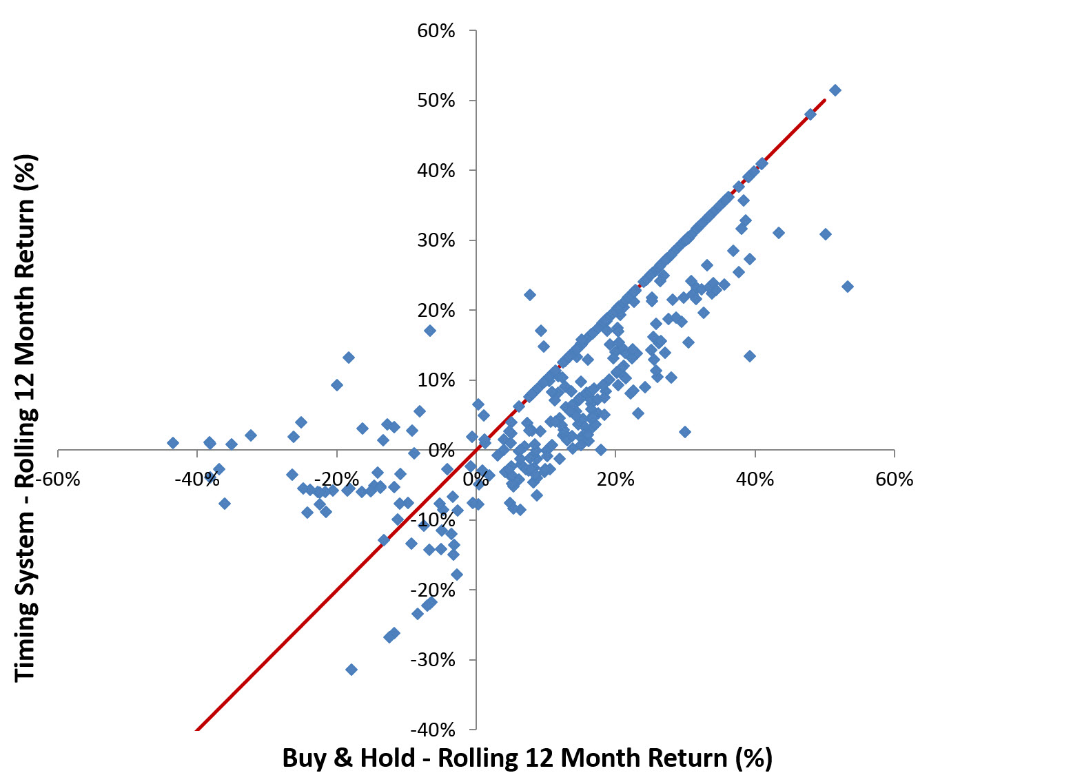
Figure 4 shows a plot of 12-month TF performance for a 100-day channel breakout system applied to the S&P 500, versus 12-month buy and hold performance. The resulting profile looks a lot like a very messy call option payout, with the left tail (highly negative returns) significantly reduced on average, but not by a predefined amount. Similarly, in bull markets, often TF returns come up short of the buy and hold performance due to the whipsaw cost.
Since trend following is fundamentally liquidity demanding, with most systems buying and selling during similar times and prices, we can expect TF success to be highly sensitive to how much money is engaged in the process. After years like 1987 and 2008-2009, we can expect trend-following funds to become very popular, which leads to large money inflows and assets under management (AUM) growth. When this strategy has “too much assets,” I’d expect the whipsaw frequency and cost to increase over time, although no one knows how much industry-wide AUM leads to this sort of performance detriment.
After a long periods of underperformance, we expect money to leave this space and performance to eventually improve. Over the long term, we expect this cycle to ebb and flow, leading to a return-risk profile near the stock-cash line.
While not shown, there’s no reason to expect different performance when applying trend-following to ETFs invested in bonds, REITs and foreign stocks.
Figure 4: Simulated trend-following rolling 12-month returns versus buy and hold returns, using the 100-day channel breakout system applied to the S&P 500 Index from 1984 to 2014
Trend Following as an Attractive Investment Discipline for Investors
Trend following as applied to the stock and bond markets is an investment discipline, not an alpha-generating strategy. TF modifies the return profile by cutting extremely negative returns, but also reducing the average return, which is basically a long-term call option payout structure. Zvi Bodie, a Boston University professor, has suggested this sort of investment approach, actually combining a one-year S&P 500 call option while putting the rest of the portfolio in TIPS.2 With his approach, the investor must be willing to pay the up-front call option price, rather than let the market’s zigs and zags determine the price of bear market insurance.
The primary benefit of a trend-following market-timing approach is psychological. If you’re in the markets long enough, there will be a few extremely serious bear markets to weather. There is nothing about an efficient markets view that prevents equity indexes from falling 50-90% in value. During the Great Depression, from peak in 1929 to trough in 1932, stocks lost about 90% of their value. There is so much pain associated with those sorts of losses, it’s not surprising that some investors may give up on stocks forever.
There are many historical moments when stock markets fell by 60 to 80% in value. This sort of thing happens in emerging markets all the time. The trend-following approach is about as simple as it gets with respect to offering reasonably robust loss minimization for these sorts of markets. Other approaches, such as relying on market gurus or using multi-parameter, optimized timing systems to call tops, have always come up short in the long run compared to the trend-following approach.
An additional risk faced by investors is a secular bear market, which is loosely defined as a 10 to 15 year period of subpar or below-inflation stock market returns. According to Ned Davis Research (Report T_202.RPT)1, past periods for the S&P 500 include 2000 to 2009, 1966 to 1982, 1929 to 1942 and 1906 to 1921. In secular bear markets, I expect trend following to enhance returns and greatly reduce losses since during these periods, cyclical bear markets are typically more frequent and longer. Another example of a secular bear market is the Japanese Nikkei 225, which continues to languish 50% below its peak set in late 1989.
Trend Following as an Attractive Investment Discipline for Asset Class Traders
For an asset class trader, there are additional benefits. While trend following reduces returns over the long term, a good asset class trader will use various trading edges to push the risk-return profile back above the stock-cash line and the stock-bond line – in essence, using trading edges to pay for the bear-market insurance. As stated before, the goal of this blog is to figure out what works in finding such asset class trading edges.
Trend following is also very attractive in taking a 50% equity decline off the table. In addition, TF supplies a lot of cash, or dry powder, to exploit the many trading opportunities revolving around providing liquidity to the market in times of crisis. Having a portfolio that is mostly in cash while markets are crashing is a position of strength psychologically to exploit opportunities created by the motivated and panic selling. I’m guessing that nothing is more frustrating for a portfolio manager than to be fully invested while stocks are tanking, or worse, faced with redemptions during a time when investment and trading opportunities are rich.
References
- Ned Davis Research, ndr.com. (Subscription required.)
- Bodie, M.J. Clowes, Worry-Free Investing: A Safe Approach to Achieving Your Lifetime Financial Goals, 2003.
Disclosure for Backtested Studies
- Trend-following models applied to S&P 500 total return index.
- No transaction fees.
- Trades initiated at the close of the next day following the buy/sell signal.
- S&P 500 total return data from:
- SPDR S&P 500 ETF (Symbol: SPY) back to January 1, 1993.
- S&P 500 total return series constructed from S&P 500 Index and daily yield data. Data from S&P.
- T-bill data from http://www.federalreserve.gov/releases/H15/data.htm. Used three-month T-bill (secondary market) daily yield to calculate cash returns.
- Barclays Aggregate Bond Index monthly data from Morningstar.
- Stock-bond and stock-cash lines assume yearly rebalancing various mixes in 5% increments.
Disclosure
The content contained within this blog reflects the personal views and opinions of Dennis Tilley, and not necessarily those of Merriman Wealth Management, LLC. This website is for educational and/or entertainment purposes only. Use this information at your own risk, and the content should not be considered legal, tax or investment advice. The views contained in this blog may change at any time without notice, and may be inappropriate for an individual’s investment portfolio. There is no guarantee that securities and/or the techniques mentioned in this blog will make money or enhance risk-adjusted returns. The information contained in this blog may use views, estimates, assumptions, facts and information from other sources that are believed to be accurate and reliable as of the date of each blog entry. The hypothetical data displayed in this blog does not represent actual performance and should not be interpreted as an indication of actual performance. Although we have done our best to present this information fairly, hypothetical performance is still potentially misleading. This data is based on transactions that were not made. Instead, the trades were simulated, based on knowledge that was available only after the fact and thus with the benefit of hindsight. Results do not include the impact of taxes, if any. The content provided within this blog is the property of Dennis Tilley & Merriman Wealth Management, LLC (“Merriman”). For more details, please consult the Important Disclosure link here.